Homepage

European Microscopy Congress 2020 Abstract Database

Quantitative Analysis of Intensity Attenuation with Increasing Thickness in TEM and STEM Images

Quantitative Analysis of Intensity Attenuation with Increasing Thickness in TEM and STEM Images

Session

PST.6 - In-situ and in-operando microscopy

Authors

Dr. Jun Yamasaki (3, 2), Mr. Yuya Ubata (3), Dr. Hideo Nishikubo (1), Dr. Hirokazu Sasaki (1), Dr. Shigeo Arai (2), Prof. Hidehiro Yasuda (3)

Affiliations

1. Furukawa Electric Co., Ltd.
2. Nagoya University
3. Osaka University

Keywords

electron transmission attenuation

high-voltage electron microscope

mass-thickness contrast

multiple scattering

Abstract text

The capability to observe a thick specimen should be important for not only efficient and reliable analyses of defects distributions in bulk but also electron tomography of micron-sized materials [1] and in-situ observations in gas or liquid environments. Deep understanding of the electron transmission feature is one of the important issues to estimate the observable thickness and to make efficient designing of those experimental researches. In the present study, the transmission attenuations were precisely analyzed using 200keV–3MeV electron beams for several amorphous materials [2].

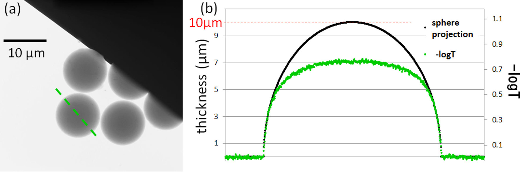
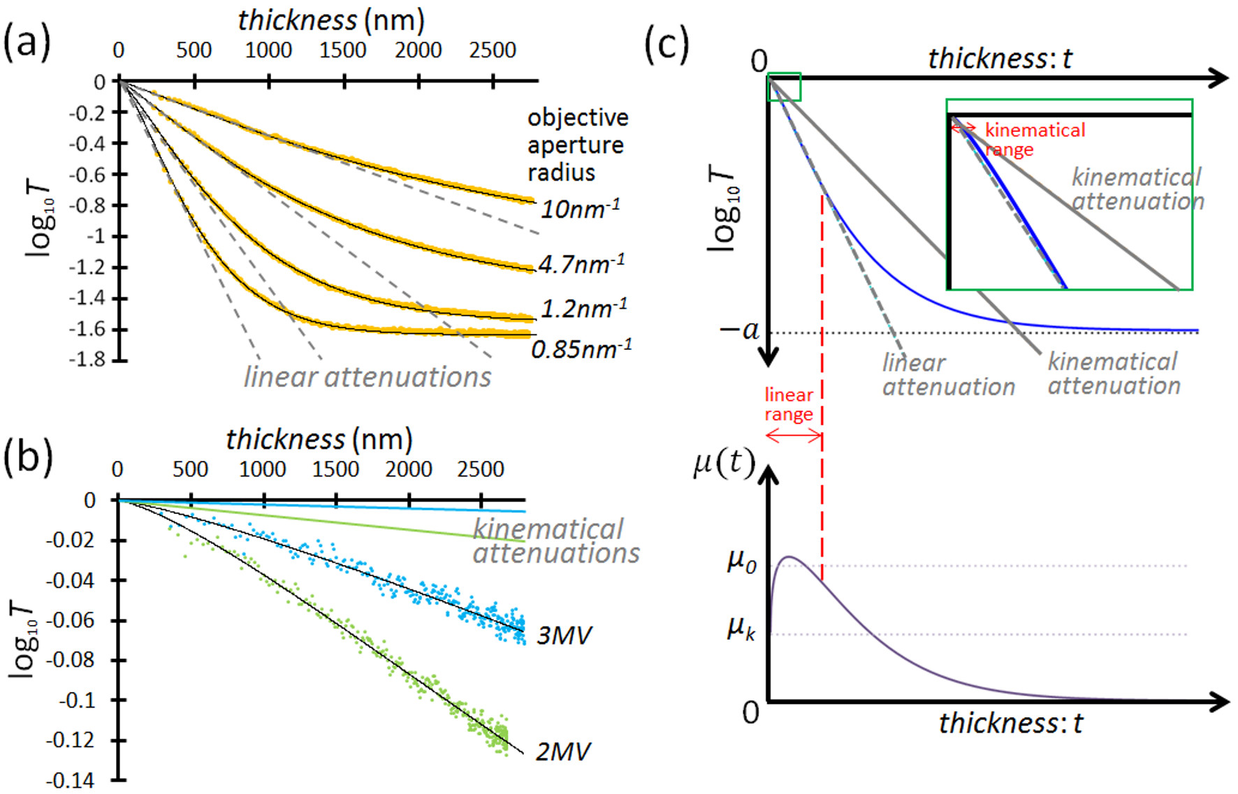
Figure 1 explains the procedure to measure the relation between the transmission T and thickness t. After measuring the intensity of a polystyrene sphere along the dashed line in Fig. 1(a), the intensity profile is normalized by that of the surrounding area to make the transmission profile. Figure 1(b) shows a comparison between the log₁₀T profile and thickness profile calculated for the sphere. Then the relation between them was converted to the attenuation curve as shown in Fig. 2(a). The same procedure is applicable to other amorphous materials with well-defined 3D shapes such as amorphous carbon microcoils [1] and wedge-shaped NiP fabricated by focused ion beams. Figure 2(a) shows the transmission attenuations for 200 keV electrons observed with various objective aperture sizes. If a material is thin enough for the kinematical approximation of electron scattering, it is generally considered that the transmission shows an exponential decay with increasing thickness (Beer’s law), resulting in a straight line in the log₁₀T chart. Thus the attenuation curves in thick materials shown in Fig. 2(a) are results from multiple scatterings [1]. In addition, also in the early stage of the attenuations, not a linear but a slight convex feature was found as shown in Fig. 2(b). This should be a quite unanticipated result which means breakdown of Beer’s law even in the early stage of the transmission attenuation.

Figure 1. Measurements of the electron transmission. (a) TEM image of polystyrene spheres. (b) Comparison between the transmission and projected thickness of a sphere.

To express the nonlinear attenuation curves, we proposed a function containing three parameters. The function was compared with the intensity attenuation in TEM images of polystyrene and amorphous carbon and STEM images of NiP in a 200-kV and high-voltage electron microscopes at Osaka University and Nagoya University over a wide range of conditions: acceleration voltage of 200kV–3MV, acceptance angles of 0.85–30 nm^-1, and thickness of 0.25–10 μm [2]. As shown in Fig. 2(a) and (b), all the experimental data are successfully reproduced by the function with high degrees of precision. Figure 2(c) schematically shows the overall shape of a typical attenuation curve and the corresponding derivative, that is, the attenuation coefficient μ(t) as a function of thickness. Although the linear attenuation tends to be considered as a kinematical scattering phenomenon, it is clearly shown in Fig. 2(c) that the linear attenuation with a coefficient of μ₀ is not directly related to the kinematical attenuation with μ_k. The characteristic behavior of the attenuation curves can be explained based on a simplified model of multiple scattering [2].

Figure 2. The transmission attenuation curves for polystyrene measured by (a) 200-keV and (b) 2 and 3-MeV electrons. The solid black curves show the fitting results by the proposed function. (c) Schematic diagrams of the attenuation curve (upper) and the attenuation coefficient (lower) depending on thickness. μ_k and μ₀ are the stationary coefficients for the kinematical and linear attenuations, respectively.

References

[1] J. Yamasaki, et al., Microscopy 63 (2014) p. 345.

[2] J. Yamasaki, Y. Ubata and H. Yasuda, Ultramicroscopy 200 (2019) p. 20.

[3] The authors are grateful to Prof. H. Mori for invaluable discussion and Mr. E. Taguchi, Dr. T. Sakata and Mr. T. Yasuda of Osaka university, and Mr. A. Ohsaki, Dr. S. Ohta, and Mr. S. Takakuwa of JEOL Co., Ltd. for their assistance with the experiments. This work was partly supported by MEXT KAKENHI (grant number 26105009).